Wigner quasi-probability distribution
- See also Wigner distribution, a disambiguation page.
The Wigner quasi-probability distribution (also called the Wigner function or the Wigner–Ville distribution after Eugene Wigner and Jean-André Ville) is a quasi-probability distribution. It was introduced by Eugene Wigner in 1932 to study quantum corrections to classical statistical mechanics. The goal was to link the wavefunction that appears in Schrödinger's equation to a probability distribution in phase space.
It is a generating function for all spatial autocorrelation functions of a given quantum-mechanical wavefunction ψ(x). Thus, it maps on the quantum density matrix in the map between real phase-space functions and Hermitian operators introduced by Hermann Weyl in 1927, in a context related to representation theory in mathematics (cf. Weyl quantization in physics). In effect, it is the Weyl–Wigner transform of the density matrix, so the realization of that operator in phase space. It was later rederived by Jean Ville in 1948 as a quadratic (in signal) representation of the local time-frequency energy of a signal.
In 1949, José Enrique Moyal, who had derived it independently, recognized it as the quantum moment-generating functional, and thus as the basis of an elegant encoding of all quantum expectation values, and hence quantum mechanics, in phase space (cf Weyl quantization). It has applications in statistical mechanics, quantum chemistry, quantum optics, classical optics and signal analysis in diverse fields such as electrical engineering, seismology, biology, speech processing, and engine design.
Relation to classical mechanics
A classical particle has a definite position and momentum, and hence it is represented by a point in phase space. Given a collection (ensemble) of particles, the probability of finding a particle at a certain position in phase space is specified by a probability distribution, the Liouville density. This strict interpretation fails for a quantum particle, due to the uncertainty principle. Instead, the above quasi-probability Wigner distribution plays an analogous role, but does not satisfy all the properties of a conventional probability distribution; and, conversely, satisfies boundedness properties unavailable to classical distributions.
For instance, the Wigner distribution can and normally does go negative for states which have no classical model—and is a convenient indicator of quantum mechanical interference. Smoothing the Wigner distribution through a filter of size larger than ħ (e.g., convolving with a phase-space Gaussian to yield the Husimi representation, below), results in a positive-semidefinite function, i.e., it may be thought to have been coarsened to a semi-classical one. (Specifically, since this convolution is invertible, in fact, no information has been sacrificed, and the full quantum entropy has not increased, yet. However, if this resulting Husimi distribution is then used as a plain measure in a phase-space integral evaluation of expectation values without the requisite star product of the Husimi representation, then, at that stage, quantum information has been forfeited and the distribution is a semi-classical one, effectively. That is, depending on its usage in evaluating expectation values, the very same distribution may serve as a quantum or a classical distribution function.)
Regions of such negative value are provable (by convolving them with a small Gaussian) to be "small": they cannot extend to compact regions larger than a few ħ, and hence disappear in the classical limit. They are shielded by the uncertainty principle, which does not allow precise location within phase-space regions smaller than ħ, and thus renders such "negative probabilities" less paradoxical.
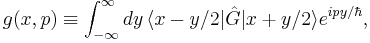
Definition and meaning
The Wigner distribution P(x, p) is defined as:
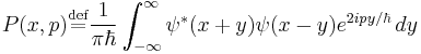
where ψ is the wavefunction and x and p are position and momentum but could be any conjugate variable pair. (i.e. real and imaginary parts of the electric field or frequency and time of a signal). Note it may have support in x even in regions where ψ has no support in x ("beats").
It is symmetric in x and p:
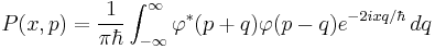
where φ is the Fourier transform of ψ.
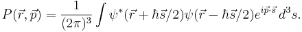
In 3D,
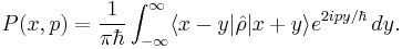
In the general case, which includes mixed states, it is the Wigner transform of the density matrix:
This Wigner transformation (or map) is the inverse of the Weyl transform, which maps phase-space functions to Hilbert-space operators, in Weyl quantization. Thus, the Wigner function is the cornerstone of quantum mechanics in phase space.
In 1949, José Enrique Moyal elucidated how the Wigner function provides the integration measure (analogous to a probability density function) in phase space, to yield expectation values from phase-space c-number functions g(x,p) uniquely associated to suitably ordered operators  through Weyl's transform (cf. Weyl quantization and property 7 below), in a manner evocative of classical probability theory.
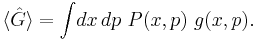
Specifically, an operator's expectation value is a "phase-space average" of the Wigner transform of that operator,
Mathematical properties
1. P(x, p) is real
2. The x and p probability distributions are given by the marginals:
 If the system can be described by a pure state, one gets
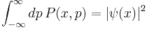
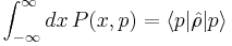 . If the system can be described by a pure state, one has
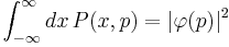
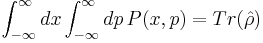
- Typically the trace of ρ is equal to 1.
- 1. and 2. imply that P(x, p) is negative somewhere, with the exception of the coherent state (and mixtures of coherent states) and the squeezed coherent state.
3. P(x, p) has the following reflection symmetries:
- Time symmetry:

- Space symmetry:

4. P(x, p) is Galilei-covariant:

- It is not Lorentz covariant.
5. The equation of motion for each point in the phase space is classical in the absence of forces:
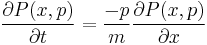
In fact, it is classical even in the presence of harmonic forces.
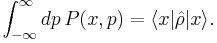
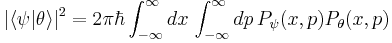
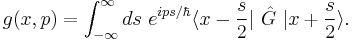
6. State overlap is calculated as:
7. Operator expectation values (averages) are calculated as phase-space averages of the respective Wigner transforms:

8. In order that P(x, p) represent physical (positive) density matrices:
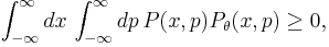
where |θ> is a pure state.
9. By virtue of the Cauchy–Schwarz inequality, for a pure state, it is constrained to be bounded,
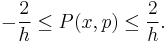
This bound disappears in the classical limit, ħ → 0. In this limit, P(x, p) reduces to the probability density in coordinate space x, usually highly localized, multiplied by δ-functions in momentum: the classical limit is "spiky". Thus, this quantum-mechanical bound precludes a Wigner function which is a perfectly localized delta function in phase space, as a reflection of the uncertainty principle.
The Wigner–Weyl transformation
The Wigner transformation is a general transformation of an operator  on a Hilbert space to a function g(x,p) on phase space and is given by
Hermitean operators map to real functions. The inverse of this transformation, so from phase space to Hilbert space, is called the Weyl transformation,
(not to be confused with another definition of the Weyl transformation). The Wigner function discussed here is the Wigner transform of the density matrix operator, so the trace of an operator with the density matrix Wigner transforms to the phase-space integral overlap of g(x, p) with the Wigner function.
Evolution equation for Wigner function
The Wigner transform of the von Neumann equation of the density matrix is Moyal's evolution equation for the Wigner function,
where H(x,p) is Hamiltonian and { {• , •} } is the Moyal bracket. In the classical limit ħ → 0, the Moyal bracket reduces to the Poisson bracket, while this evolution equation reduces to the Liouville equation of classical statistical mechanics.
Formally, in terms of quantum characteristics, the solution of this evolution equation reads,

where  and
and  are solutions of so-called quantum Hamilton's equations, subject to initial conditions
  and
and  , and where ∗-product composition is understood for all argument functions. Nevertheless, in practice, evaluating such expressions is cumbersome, and concepts of classical trajectories hardly cross over to the quantum domain, as the "quantum probability fluid" diffuses, and, with few exceptions, the classical trajetory is barely discernible in an evolving Wigner distribution function.
Uses of the Wigner function outside quantum mechanics
- In the modelling of optical systems such as telescopes or fibre telecommunications devices, the Wigner function is used to bridge the gap between simple ray tracing and the full wave analysis of the system. Here p/ħ is replaced with k = |k|sinθ ≈ |k|θ in the small angle (paraxial) approximation. In this context, the Wigner function is the closest one can get to describing the system in terms of rays at position x and angle θ while still including the effects of interference. If it becomes negative at any point then simple ray-tracing will not suffice to model the system.
- In signal analysis, a time-varying electrical signal, mechanical vibration, or sound wave are represented by a Wigner function. Here, x is replaced with the time and p/ħ is replaced with the angular frequency ω = 2πf, where f is the regular frequency.
- In ultrafast optics, short laser pulses are characterized with the Wigner function using the same f and t substitutions as above. Pulse defects such as chirp (the change in frequency with time) can be visualized with the Wigner function. See Figure 2.
- In quantum optics, x and p/ħ are replaced with the X and P quadratures, the real and imaginary components of the electric field (see coherent state). The plots in Figure 1 are of quantum states of light.
Measurements of the Wigner function
- Tomography
- Homodyne detection
- FROG Frequency-resolved optical gating
The Wigner distribution was the first quasi-probability distribution to be formulated, but many more followed, formally equivalent and transformable to and from it (cf. Cohen's class distribution function). As in the case of coordinate systems, on account of varying properties, several such have with various advantages for specific applications:
Nevertheless, The Wigner distribution holds, in some sense, a privileged position among all these distributions, since it is the only one whose requisite star product drops out (integrates out by parts to effective unity) in the evaluation of expectation values, as illustrated above, and so can be visualized as a quasi-probability measure analogous to the classical ones.
Historical note
As indicated, the formula for the Wigner function was independently derived several times in different contexts. In fact, apparently, Wigner was unaware that even within the context of quantum theory, it had been introduced previously by Heisenberg and Dirac, albeit purely formally: these two missed its significance, and that of its negative values, as they merely considered it as an approximation to the full quantum description of a system such as the atom. (Incidentally, Dirac would later become Wigner's brother-in-law.) Symmetrically, in most of his legendary 18-month correspondence with Moyal in the mid 1940s, Dirac was unaware that Moyal's quantum-moment generating function was effectively the Wigner function, and it was Moyal who finally brought it to his attention.
See also
- Heisenberg group
- Weyl quantization
- Moyal bracket
- Modified Wigner distribution function
- Negative probability
- Cohen's class distribution function
- Wigner distribution function
References
- E.P. Wigner, "On the quantum correction for thermodynamic equilibrium", Phys. Rev. 40 (June 1932) 749–759. doi:10.1103/PhysRev.40.749
- H. Weyl, Z. Phys. 46, 1 (1927). doi:10.1007/BF02055756
- H. Weyl, Gruppentheorie und Quantenmechanik (Leipzig: Hirzel) (1928).
- H. Weyl, The Theory of Groups and Quantum Mechanics (Dover, New York, 1931).
- H.J. Groenewold, "On the Principles of elementary quantum mechanics",Physica,12 (1946) 405–460. doi:10.1016/S0031-8914(46)80059-4
- J. Ville, "Théorie et Applications de la Notion de Signal Analytique", Câbles et Transmission, 2, 61–74 (1948).
- J.E. Moyal, "Quantum mechanics as a statistical theory", Proceedings of the Cambridge Philosophical Society, 45, 99–124 (1949). doi:10.1017/S0305004100000487
- W. Heisenberg, "Über die inkohärente Streuung von Röntgenstrahlen", Physik. Zeitschr. 32, 737–740 (1931).
- P.A.M. Dirac, "Note on exchange phenomena in the Thomas atom", Proc. Camb. Phil. Soc. 26, 376–395 (1930).
- C. Zachos, D. Fairlie, and T. Curtright, Quantum Mechanics in Phase Space ( World Scientific, Singapore, 2005) ISBN 978-981-238-384-6 .
- Gallery of rotating Wigner Functions
- Gallery of WFs
- Quantum Optics Gallery
- M. Levanda and V Fleurov, "Wigner quasi-distribution function for charged particles in classical electromagnetic fields", Annals of Physics, 292, 199–231 (2001). http://arxiv.org/abs/cond-mat/0105137
- Wigner Distribution Function and its relationship with geometric optics